Probability

Probability

Sample space Ω: The set of all the outcomes of a random experiment
Event space F: A set whose elements A ∈ F (called events) are subsets of Ω $P ( A ) \geq 0 , \text { for all } A \in \mathcal { F }$ $P ( \Omega ) = 1$ $\sum _ { i = 1 } ^ { k } P \left( A _ { k } \right) = 1$

The conditional probability of any event A given B is defined as

$$P ( A | B ) \triangleq \frac { P ( A \cap B ) } { P ( B ) }$$

a random variable X is a function X: $\Omega \longrightarrow \mathbb { R } ^ { 2 }$

A cumulative distribution function (CDF) $F _ { X } ( x ) \triangleq P ( X \leq x )$

Cumulative distribution function(CDF)

Probability mass functions: When a random variable X is a discrete then

$$p _ { X } ( x ) \triangleq P ( X = x )$$ $$0 \leq p _ { X } ( x ) \leq 1$$

Probability density functions - For some continuous random variables, the cumulative distribution function F(x)is differentiable everywhere. $f _ { X } ( x ) \triangleq \frac { d F _ { X } ( x ) } { d x }$ $\int _ { - \infty } ^ { \infty } f _ { X } ( x ) = 1$

Expectation

If X is a discrete random variable with PMF $p _ { X } ( x ) \text { and } g : \mathbb { R } \longrightarrow \mathbb { R }$, then expected value $E [ g ( X ) ] \triangleq \sum _ { x \in V a l ( X ) } g ( x ) p _ { X } ( x )$

For continuous randon variable

$$E [ g ( X ) ] \triangleq \int _ { - \infty } ^ { \infty } g ( x ) f _ { X } ( x ) d x$$

This is also known as the mean of the random variable X

Variance

The variance of a random variable X is a measure of how concentrated the distribution of a random variable X is around its mean

$$\operatorname { Var } [ X ] \triangleq E \left[ ( X - E ( X ) ) ^ { 2 } \right]$$

Some common Discrete random variables

X ~ Binomial(n,p) (where $0 \leq p \leq 1$ ): the number of heads in n independent flips of a coin with heads probability p.

$$p ( x ) = \left( \begin{array} { l } { n } \\ { x } \end{array} \right) p ^ { x } ( 1 - p ) ^ { n - x }$$

X ~ Poisson($\lambda$) (where $\lambda > 0$): a probability distribution over the nonnegative integers used for modeling the frequency of rare events

$$p ( x ) = e ^ { - \lambda } \frac { \lambda ^ { x } } { x ! }$$

some common continuous random variable

1. X ~ Uniform(a,b) (where a < b): equal probability density to every value between a and b on the real line. $f ( x ) = \left\{ \begin{array} { l l } { \frac { 1 } { b - a } } & { \text { if } a \leq x \leq b } \\ { 0 } & { \text { otherwise } } \end{array} \right.$
2. $X \sim \operatorname { Normal } \left( \mu , \sigma ^ { 2 } \right)$ also known as the Gaussian distribution $f ( x ) = \frac { 1 } { \sqrt { 2 \pi } \sigma } e ^ { - \frac { 1 } { 2 \sigma ^ { 2 } } ( x - \mu ) ^ { 2 } }$

Gaussian distribution

Uniform distribution

Mean and Variance of common probability functions

Joint and marginal probability mass functions

Joint probability mass function $p _ { X Y } ( x , y ) = P ( X = x , Y = y )$

Marginal probability mass function $p _ { X } ( x ) = \sum _ { y } p _ { X Y } ( x , y )$

Joint probability density function $f _ { X Y } ( x , y ) = \frac { \partial ^ { 2 } F _ { X Y } ( x , y ) } { \partial x \partial y }$

Marginal probability density function $f _ { X } ( x ) = \int _ { - \infty } ^ { \infty } f _ { X Y } ( x , y ) d y$

Conditional PMF $p _ { Y

X } ( y

x ) = \frac { p _ { X Y } ( x , y ) } { p _ { X } ( x ) }$

Conditional PDF $f _ { Y

X } ( y

x ) = \frac { f _ { X Y } ( x , y ) } { f _ { X } ( x ) }$

Two random variables X and Y are independent if $p _ { X Y } ( x , y ) = p _ { X } ( x ) p _ { Y } ( y )$ for discrete case and $F _ { X Y } ( x , y ) = F _ { X } ( x ) F _ { Y } ( y )$ for continuous case

Chain Rule

$f \left( x _ { 1 } , x _ { 2 } , \ldots , x _ { n } \right)$ $= f \left( x _ { 1 } \right) \prod _ { i = 2 } ^ { n } f \left( x _ { i }

x _ { 1 } , \ldots , x _ { i - 1 } \right)$

Bayes Rule

Discrete Case $P _ { Y

X } ( y

x ) = \frac { P _ { X Y } ( x , y ) } { P _ { X } ( x ) } = \frac { P _ { X

Y } ( x

y ) P _ { Y } ( y ) } { \sum _ { y ^ { \prime } \in V a l ( Y ) } P _ { X

Y } ( x

y ^ { \prime } ) P _ { Y } \left( y ^ { \prime } \right) }$

Continuous Case $f _ { Y

X } ( y

x ) = \frac { f _ { X Y } ( x , y ) } { f _ { X } ( x ) } = \frac { f _ { X

Y } ( x

y ) f _ { Y } ( y ) } { \int _ { - \infty } ^ { \infty } f _ { X

Y } ( x

y ^ { \prime } ) f _ { Y } \left( y ^ { \prime } \right) d y ^ { \prime } }$

To study the relationship of two random variables with each other we use the covariance

$$\operatorname { Cov } [ X , Y ] \triangleq E [ ( X - E [ X ] ) ( Y - E [ Y ] ) ]$$

Covariance matrix: is the square matrix whose entries are given by $\Sigma _ { i j } = \operatorname { Cov } \left[ X _ { i } , X _ { j } \right]$

Normalizing the covariance gives the correlation

$$\rho ( X , Y ) = \frac { \operatorname { Cov } ( X , Y ) } { \sqrt { \operatorname { Var } ( X ) \operatorname { Var } ( Y ) } }$$

Correlation also measures the linear relationship between two variables, but unlike covariance always lies between−1 and 1

Multivariate Gaussian distribution

$$f _ { X _ { 1 } , X _ { 2 } , \ldots , X _ { n } } \left( x _ { 1 } , x _ { 2 } , \ldots , x _ { n } ; \mu , \Sigma \right) = \frac { 1 } { ( 2 \pi ) ^ { n / 2 } | \Sigma | ^ { 1 / 2 } } \exp \left( - \frac { 1 } { 2 } ( x - \mu ) ^ { T } \Sigma ^ { - 1 } ( x - \mu ) \right)$$

Maximum likelihood estimation(MLE)

MLE is to choose parameters that “explain” the data best by maximizing the probability/density of the data we’ve seen as a function of the parameters.

$\hat { \theta } _ { \mathrm { MLE } } = \underset { \theta } { \arg \max } \mathcal { L } ( \theta )$ where $\mathcal { L }$ is the likelihood function. $\mathcal { L } ( \theta ) = p \left( x _ { 1 } , \ldots , x _ { n } ; \theta \right)$

It is usually convenient to take logs, giving rise to the log-likelihood.

$$\log \mathcal { L } ( \theta ) = \sum _ { i = 1 } ^ { n } \log p \left( x _ { i } ; \theta \right)$$

Let us derive a simple example for a coin toss model where m = no of successes and N = Number of coin flips

For a Bernoulli distribution

$$p \left( x _ { i }	\theta \right) = \theta ^ m ( 1 - \theta ) ^ {n-m }$$
$$p \left( x _ { i }	\theta \right) =\prod _ { i = 1 } ^ { n } \left( \theta ^ m \right) ( 1 - \theta ) ^ { n-m }$$

Log likelihood is

$$\ell ( \theta )= \log P \left( x _ { 1 } : { n } | \theta \right) = m \log \theta + ( n - m ) \log ( 1 - \theta )$$

Differentiate and Equate to Zero to find $\theta$

$$\frac { d \ell (\theta ) } { d \theta } = \frac { d } { d \theta } ( m \log \theta + ( n - m ) \log ( 1 - \theta ) )$$ $$= \frac { m } { \theta } + ( n - m ) ( - 1 ) \frac { 1 } { 1 - \theta }$$ $$= \frac { ( 1 - \theta ) m + ( n - n ) \theta } { \theta ( 1 - \theta ) } = 0$$ $$m - \theta m + \theta m - \theta n = 0$$ $$\theta = m / n$$

Maximum a posteriori estimation(MAP)

We assume that the parameters are a random variable, and we specify a prior distribution p(θ).

Using Bayes rule $p ( \theta

x _ { 1 } , \ldots , x _ { n } ) \propto p ( \theta ) p \left( x _ { 1 } , \ldots , x _ { n }

\theta \right)$

We can ignore the Normalizing constant as it does not affect the MAP estimate.

$$\hat { \theta } _ { \mathrm { MAP } } = \underset { \theta } { \arg \max } p ( \theta ) p \left( x _ { 1 } , \ldots , x _ { n } | \theta \right)$$

If the observations are iid (independent and identically distributed) then

$$\hat { \theta } _ { \mathrm { MAP } } = \underset { 0 } { \arg \max } \left( \log p ( \theta ) + \sum _ { i = 1 } ^ { n } \log p \left( x _ { i } | \theta \right) \right)$$

Example MAP for Bernoulli Coin Toss

The likelihood is as follows given that there are m successes and n trials

$$p \left( x _ { 1 : n } | \theta \right) = \theta ^ { m } ( 1 - \theta ) ^ { n - m }$$

We need to specify prior. For Bernoulli distribution we use Beta distribution which is the conjugate prior.

$$P(\theta)=\frac { \Gamma( \alpha + \beta ) } { \Gamma( \alpha ) \Gamma ( \beta ) }\theta ^ { \alpha - 1 } ( 1 - \theta ) ^ { \beta - 1 }$$

Now we can compute the posterior
$p ( \theta | x _ { 1 : n } ) \propto p \left( x _ { 1 : n } | \theta \right) p ( \theta )$

$$= \theta ^ { m } ( 1 - \theta ) ^ { n - m } \theta ^ { \alpha - 1 } ( 1 - \theta ) ^ { \beta - 1 }$$ $$= \theta ^ { m + \alpha - 1 } ( 1 - \theta ) ^ { n - m + \beta - 1 }$$ $$p ( \theta | x _ { 1 : n } ) =\frac { \Gamma \left( \alpha ^ { \prime } + b ^ { \prime } \right) } { \Gamma \left( \alpha ^ { \prime } \right) \Gamma \left( \beta ^ { \prime } \right) }\theta ^ { \alpha ^ { \prime } - 1 } ( 1 - \theta ) ^ { \beta^\prime - 1 }$$

Information Theory

We can quantify the amount of uncertainty in an entire probability distribution using the Shannon entropy of an event X = x

$$H ( \mathrm { x } ) = \mathbb { E } _ { \mathrm { x } \sim P } [ I ( x ) ] = - \mathbb { E } _ { \mathrm { x } \sim P } [ \log P ( x ) ]$$

If we have two separate probability distributions P (x) and Q (x) over the same random variable x, we can measure how different these two distributions are using the Kullback-Leibler (KL) divergence:

$$D _ { \mathrm { KL } } ( P \| Q ) = \mathbb { E } _ { \mathrm { x } \sim P } \left[ \log \frac { P ( x ) } { Q ( x ) } \right] = \mathbb { E } _ { \mathrm { x } \sim P } [ \log P ( x ) - \log Q ( x ) ]$$

The KL divergence has many useful properties, most notably that it is nonnegative. The KL divergence is 0 if and only if P and Q are the same distribution in the case of discrete variables, or equal “almost everywhere” in the case of continuous variables . A quantity that is closely related to the KL divergence is the cross-entropy.

$$H ( P , Q ) = - \mathbb { E } _ { \mathrm { x } \sim P } \log Q ( x )$$

Minimizing the cross-entropy with respect to Q is equivalent to minimizing the KL divergence.

Example for a Bernoulli Variable x the entropy is

$$H = - \sum _ { x _ { \mathfrak { z } } } ^ { 1 } \theta ^ { x } ( 1 - \theta ) ^ { 1 - x } \log \left[ \theta ^ { x } ( 1 - \theta ) ^ { 1 - x } \right]$$ $$= - \theta \log \theta - ( 1 - \theta ) \log ( 1 - \theta )$$

Gaussian Process(GP)

it is referred to as the infinite-dimensional extension of the multivariate normal distribution.

$$X = \left[ \begin{array} { c } { X _ { 1 } } \\ { X _ { 2 } } \\ { \vdots } \\ { X _ { n } } \end{array} \right] \sim \mathcal { N } ( \mu , \Sigma )$$

A GP is specified by a mean function m(x) and a covariance function , otherwise known as a kernel. The shape and smoothness of our function is determined by the covariance function, as it controls the correlation between all pairs of output values.

For Each partition XX and YY only depends on its corresponding entries in $\mu$ and $\Sigma$ .

$$\left[ \begin{array} { c } { X } \\ { Y } \end{array} \right] \sim \mathcal { N } ( \mu , \Sigma ) = \mathcal { N } \left( \left[ \begin{array} { c } { \mu _ { X } } \\ { \mu _ { Y } } \end{array} \right] , \left[ \begin{array} { c } { \Sigma _ { X X } \Sigma _ { X Y } } \\ { \Sigma _ { Y X } \Sigma _ { Y Y } } \end{array} \right] \right)$$

We can determine their marginalized probability distributions in the following way:

$$\begin{aligned} X & \sim \mathcal { N } \left( \mu _ { X } , \Sigma _ { X X } \right) \\ Y & \sim \mathcal { N } \left( \mu _ { Y } , \Sigma _ { Y Y } \right) \end{aligned}$$

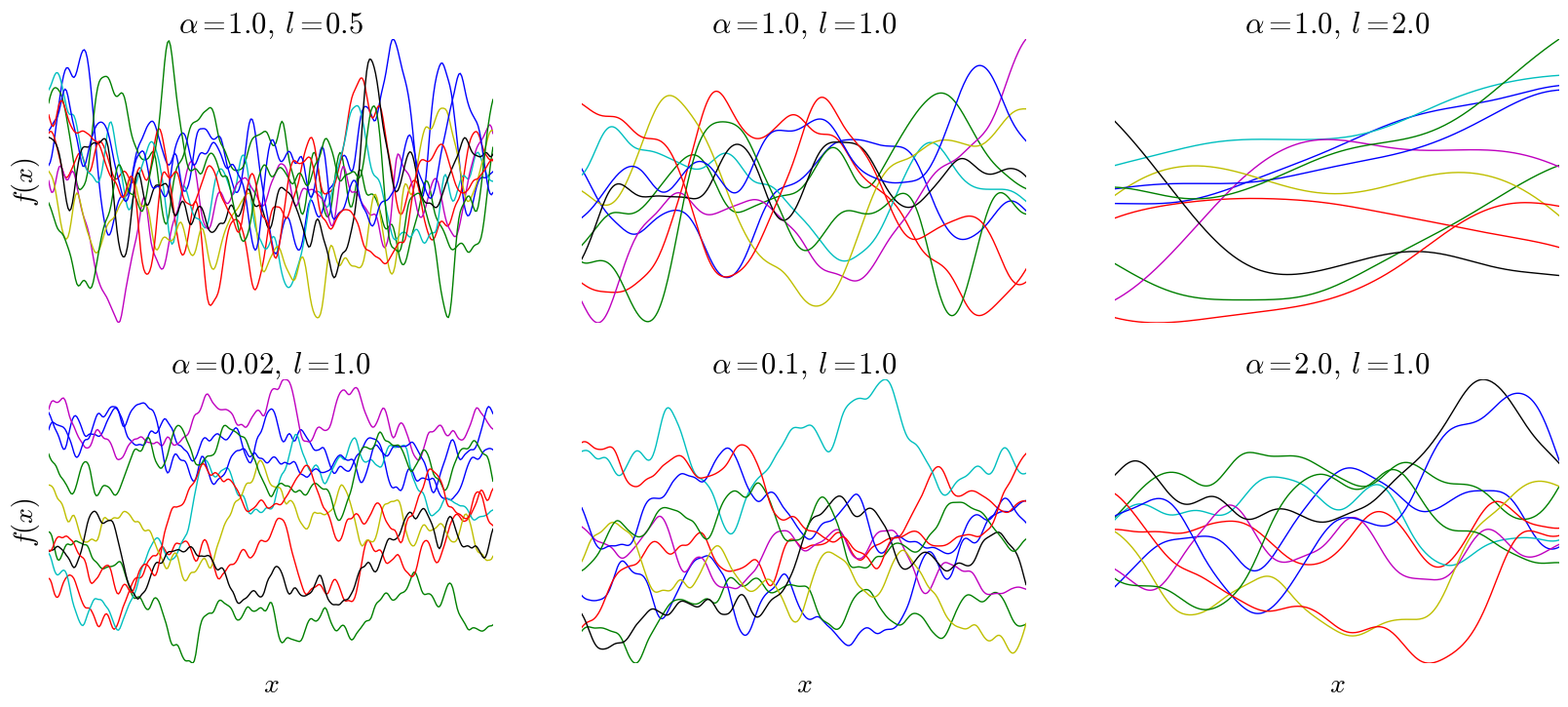
Given a mean function and a kernel, we can sample from any GP. For example, consider single-dimensional inputs $x _ { n }$ with a constant mean function at 0 and the following kernel:

$$k \left( x , x ^ { \prime } \right) = h ^ { 2 } \left( 1 + \frac { \left( x - x ^ { \prime } \right) ^ { 2 } } { 2 \alpha l ^ { 2 } } \right) ^ { - \alpha }$$

where k,α, and l are all positive real numbers, referred to as hyper-parameters. Below are samples drawn from a GP with a rational quadratic kernel and various kernel parameters, with h fixed at 1:

Samples from GP

Typically, we would like to estimate function values of a GP conditioned on some training data,

Original GP Prior and the conditioned GP on data

The GP can help estimate the uncertainty as well do non linear regression and prediction.

Inference using Monte Carlo Methods

The normalizing constant of Bayes rule is often intractable. Hence we need to use sampling methods to approximate the posterior. These are called Monte Carlo methods.

Sampling from standard distribution

The simplest method for sampling from a univariate distribution is based on the inverse probability transform. Let F be a cumulative distribution function (cdf) of some distribution we want to sample from, and let $F ^ { - 1 }$ be its inverse.

Then If $U \sim U ( 0,1 )$ is a uniform random variable then $F ^ { - 1 } ( U ) \sim F$

Sampling from inverse CDF

Markov Chain Monte Carlo(MCMC)

Rather than directly sampling from the function we construct a markov chain and sample from it to approximate the posterior

Metropolis Hastings algorithm(MH)

The basic idea in MH is that at each step, we propose to move from the current state x to a new state x′ with probability q(x′

x), where q is called the proposal distribution(also called the kernel). Having proposed a move to x′, we then decide whether to accept this proposal or not . If the proposal is accepted, the new state is x′, otherwise the new state is the same as the current state x.

$$r = \min \left( 1 , \frac { p ^ { * } \left( \mathrm { x } ^ { \prime } \right) } { p ^ { * } ( \mathrm { x } ) } \right)$$

Gibbs sampling, is a special case of MH

$$q \left( \mathbf { x } ^ { \prime } | \mathbf { x } \right) = p \left( x _ { i } ^ { \prime } | \mathbf { x } _ { - i } \right) \mathbb { I } \left( \mathbf { x } _ { - i } ^ { \prime } = \mathbf { x } _ { - i } \right)$$

We move to a new state where $x _ { i }$ is sampled from its full conditional, but $\mathbf { x } _ { - i }$ left unchanged with acceptance rate of 1 for each such proposal.

Source:Nando De Freitas

We start MCMC from an arbitrary initial state. Samples collected before the chain has reached its stationary distribution do not come from p∗, and are usually thrown away. This is called the burn-in phase.