Python Data Structure 2
Sorting
Given a collection, the goal is to rearrange the elements so that they are ordered from smallest to largest
Sorting algorithms are classified into comparison sorts (Which cannot perform better than O(n log n) in the average or worst case.) and non comparison sort
Some of the most commonly used comparison sort algorithms are merge sort and quick sort

Merge-Sort
This uses algorithmic design pattern called divide-and-conquer which consists the following steps to sort a sequence S with n elements
- Divide: S (has at least two elements) remove all the elements from S and put them into two sequences, S1 and S2, each containing about half of the elements of S
- Conquer: Recursively sort sequences S1 and S2
- Combine: Put back the elements into S by merging the sorted sequences S1 and S2 into a sorted sequence.
Algorithm merge-sort sorts a sequence S of size n in O(n log n) time, assuming two elements of S can be compared in O(1) time.
def merge_sort(nums):

if len(nums) == 1:
return

middle_index = len(nums) // 2

left_half = nums[:middle_index]
right_half = nums[middle_index:]

merge_sort(left_half)
merge_sort(right_half)

i = 0
j = 0
k = 0

while i<len(left_half) and j<len(right_half):
if left_half[i] < right_half[j]:
  nums[k] = left_half[i]
  i = i + 1
else:
  nums[k] = right_half[j]
  j = j + 1

k = k + 1

while i<len(left_half):
nums[k] = left_half[i]
k = k + 1
i = i + 1

if __name__ == "__main__":

nums = [-3,-2,-1,1,2,1,0,-1,-2,-3]
merge_sort(nums)
print(nums)
Quick-Sort
This algorithm is also based on the divide-and-conquer paradigm,
- Divide: If S has at least two elements , select a element x from S called the pivot. It is common practice to choose the pivot x to be the last element in S. Then Remove all the elements from S and put them into three sequences.
- L, storing the elements in S less than x
- E, storing the elements in S equal to x
- G, storing the elements in S greater than x
- Conquer: Recursively sort sequences L and G
- Combine: Put back the elements into S in order by first inserting the elements of L, then those of E, and finally those of G.

The running time of an execution of quick-sort as O(n · h) where h is the overall height of the quick-sort tree T for that execution. Thus quick-sort runs in O(nlogn) time.
def quick_sort(nums,low,high):

	if low >= high:
		return

	pivot_index = partition(nums,low,high)
	quick_sort(nums,low, pivot_index-1)
	quick_sort(nums, pivot_index+1,high)


def partition(nums,low,high):

	pivot_index = (low+high)//2
	swap(nums,pivot_index,high)

	i = low

	for j in range(low,high,1):
		if nums[j] <= nums[high]:
			swap(nums,i,j)
			i = i + 1

	swap(nums,i,high)

	return i

def swap(nums,i,j):
	temp = nums[i]
	nums[i] = nums[j]
	nums[j] = temp
Dynamic Programming
It refers to simplifying a complicated problem by breaking it down into simpler sub-problems in a recursive manner.
Dynamic Programming for Coin change problem
A classic example of an optimization problem involves making change using the fewest coins . For Example let us take the example of a customer gives 1 dollar and purchases for 37 cents. Assume in addition to the usual 1, 5, 10, and 25 there is also a 21 cent coin. The key to cutting down on the amount of work we do is to remember some of the past results so we can avoid recomputing results we already know. This is called memoization.
def recDC(coinValueList,change,knownResults):
   minCoins = change
   if change in coinValueList:
      knownResults[change] = 1
      return 1
   elif knownResults[change] > 0:
      return knownResults[change]
   else:
       for i in [c for c in coinValueList if c <= change]:
         numCoins = 1 + recDC(coinValueList, change-i,
                              knownResults)
         if numCoins < minCoins:
            minCoins = numCoins
            knownResults[change] = minCoins
   return minCoins

print(recDC([1,5,10,25],63,[0]*64))
Graph Algorithm
A graph is a way of representing relationships that exist between pairs of objects. Graph G is simply a set V of vertices and a collection E of pairs of vertices from V, called edges. Edges in a graph are either directed or undirected.

Data Structures for Graphs
- In an edge list, we maintain an unordered list of all edges. This minimally suffices, but there is no efficient way to locate a particular edge (u, v), or the set of all edges incident to a vertex v
- In an adjacency list, we maintain, for each vertex, a separate list containing those edges that are incident to the vertex. The complete set of edges can be determined by taking the union of the smaller sets, while the organization allows us to more efficiently find all edges incident to a given vertex.
- An adjacency map is very similar to an adjacency list, but the secondary container of all edges incident to a vertex is organized as a map, rather than as a list, with the adjacent vertex serving as a key. This allows for access to a specific edge (u, v) in O(1) expected time.
- An adjacency matrix provides worst-case O(1) access to a specific edge (u, v) by maintaining an n × n matrix, for a graph with n vertices. Each entry is dedicated to storing a reference to the edge (u, v) for a particular pair of vertices u and v; if no such edge exists, the entry will be None.

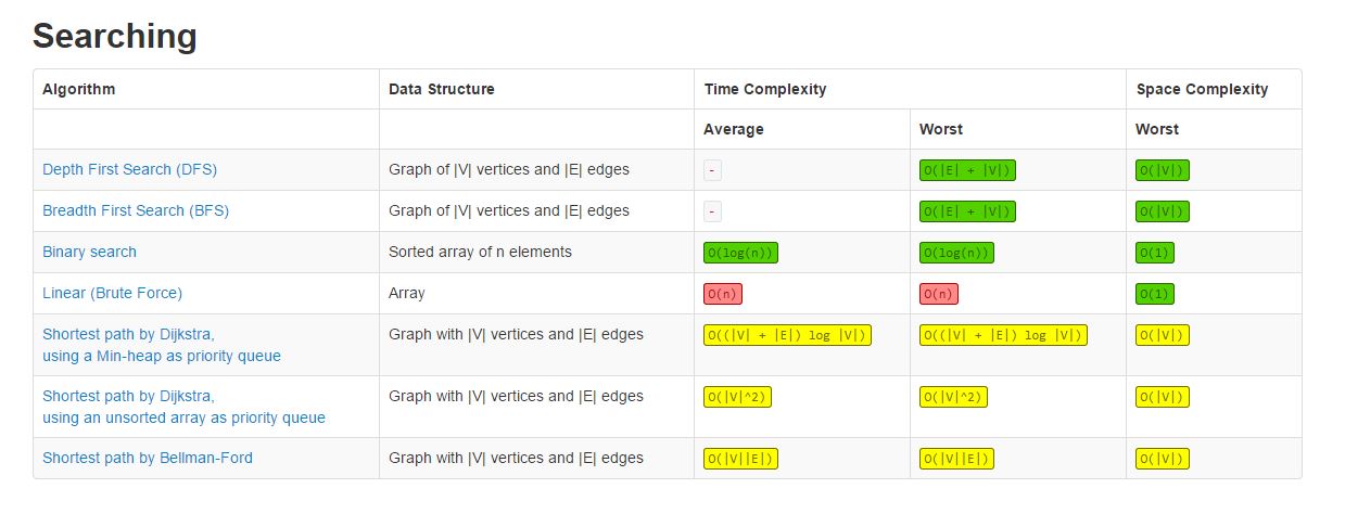
DEPTH-FIRST SEARCH(DFS)
Depth-first search is useful for testing a number of properties of graphs, including whether there is a path from one vertex to another and whether or not a graph is connected. The algorithm starts at the root node (selecting some arbitrary node as the root node in the case of a graph) and explores as far as possible along each branch before backtracking.

class Node(object):

	def __init__(self, name):
		self.name = name;
		self.adjacenciesList = [];
		self.visited = False;
		self.predecessor = None;

class DepthFirstSearch(object): # BFS -> queue + layer by layer algorithm   DFS -> stack + goes as deep aspossible into the tree !!!

	def dfs(self, node):

		node.visited = True;
		print("%s " % node.name);

		for n in node.adjacenciesList:
			if not n.visited:
				self.dfs(n);


node1 = Node("A");
node2 = Node("B");
node3 = Node("C");
node4 = Node("D");
node5 = Node("E");

node1.adjacenciesList.append(node2);
node1.adjacenciesList.append(node3);
node2.adjacenciesList.append(node4);
node4.adjacenciesList.append(node5);

dfs = DepthFirstSearch();
dfs.dfs(node1);
BREADTH-FIRST SEARCH (BFS)
Is starts at the tree root (or some arbitrary node of a graph, sometimes referred to as a ‘search key’[1]), and explores all of the neighbor nodes at the present depth prior to moving on to the nodes at the next depth level. A path in a breadth-first search tree rooted at vertex s to any other vertex v is guaranteed to be the shortest such path from s to v in terms of the number of edges.
class Node(object):

	def __init__(self, name):
		self.name = name;
		self.adjacencyList = [];
		self.visited = False;
		self.predecessor = None;

class BreadthFirstSearch(object):

	def bfs(self, startNode):

		queue = [];
		queue.append(startNode);
		startNode.visited = True;

		# BFS -> queue      DFS --> stack BUT usually we implement it with recursion !!!
		while queue:

			actualNode = queue.pop(0);
			print("%s " % actualNode.name);

			for n in actualNode.adjacencyList:
				if not n.visited:
					n.visited = True;
					queue.append(n);

node1 = Node("A");
node2 = Node("B");
node3 = Node("C");
node4 = Node("D");
node5 = Node("E");

node1.adjacencyList.append(node2);
node1.adjacencyList.append(node3);
node2.adjacencyList.append(node4);
node4.adjacencyList.append(node5);

bfs = BreadthFirstSearch();
bfs.bfs(node1);
Computational Complexity
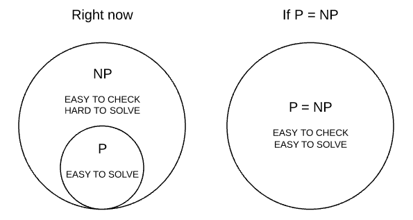
There are multiple classes for decision problems but the most famous ones are: P and NP.
P
P stands for polynomial time class, it means that the run-time of an algorithm for finding an answer in this class is considered “efficient” or “fast”.. This class contains all the problems that can be solved by a “reasonably fast” program by a deterministic Turing machine. Finding and checking an answer for an P problem is fast, independent of the size of input. These problems are called tractable, while others are called intractable or superpolynomial.
NP
NP class stands for non-Deterministic Polynomial time class. The problems in this class can be at least checked if right or wrong in polynomial time given an deterministic machine. But finding the answer takes huge time, given an huge input. Hard to find the answer, easy to check.
NP Complete
This class belongs inside NP class, it contains problems that can be reduced to others problems. If found an polynomial time answer to any problem in this class, would means that we can also find a answer in polynomial time to all NP problems. Proving P = NP. But today there’s no known efficient way to locate a solution in the first place, the most notable characteristic of NP-complete problems is that no fast solution to them is known.
A decision problem L is NP-complete if: 1) L is in NP (Any given solution for NP-complete problems can be verified quickly, but there is no efficient known solution). 2) Every problem in NP is reducible to L in polynomial time
P vs NP
If someone could find an answer in polynomial time for some NP-complete problem, it could be reduced and used the same strategy in any NP problem, meaning P = NP.